Training a sparse autoencoder
Let’s get back to experiments. We want to train an autoencoder while minimizing the sum of the L2 reconstruction loss and the L1 sparsity penalty. The theory doesn’t tell us what their relative importance should be. So the loss function is really \[ \mathrm{loss} = \mathrm{L2\_reconstruction\_loss} + \lambda \cdot \mathrm{L1\_sparsity\_penalty} \]
where \( \lambda \) is an unknown hyperparameter. If \( \lambda \) is too small, we’ve just trained a non-sparse autoencoder. If it’s too large, gradient descent will prevent any feature from ever being nonzero.
Anthropic used \( \lambda = 5 \), but the optimal value could easily differ between implementations, e.g. if we used the mean L2 reconstruction loss instead of summing it, the L1 penalty would get a larger relative weight.
So let’s run a sweep over the L1 penalty strength \( \lambda \).
Which tensor do we apply the L1 penalty to? We can’t only apply it to the feature vector
\(f \in \mathbb{R}^{10000} \).
In that case the optimizer could cheat the L1 penalty by making all the features \(f_i\) small but nonzero,
while compensating by making the elements \(C_{ij}\) of decoder_linear’s weight matrix large.
So instead we broadcast multiply \(f\) by \(C\) to get a list of 10000 feature vectors,
each one in \( \mathbb{R}^{768} \). Then we collapse each of those feature vectors into a single magnitude using
the L2 norm,
and then apply the L1 penalty to that list (call it scaled_features) of 10000 numbers.
But look at those dimensions again.
We’ve created a tensor with dimensions (768, 10000). At 4 bytes per single-precision float,
that’s ~30 megabytes. We need one such tensor per token in the training example,
so we need 6 gigabytes when the example is 200 tokens long. All of this is batch size 1.
Luckily there’s an alternative route that avoids that large tensor:
- Apply the L2 norm to collapse \(C_{ij}\) into 10000 column magnitudes
- Multiply elementwise with \(f\)
- This is the same as
scaled_features(importantly \(f_i \geq 0 \)) - Apply the L1 penalty
Tuning the L1 penalty
I trained 4 models:
- blue: \( \lambda = 0 \)
- green: \( \lambda = 5 \)
- orange: \( \lambda = 50 \)
- red: \( \lambda = 500 \)
Results of the sweep:
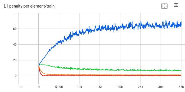
This is the L1 penalty before being multiplied by \(\lambda\)
As expected, a larger \(\lambda\) causes the L1 penalty to be smaller, since it’s more important in the loss function and hence the optimizer focuses on it more.
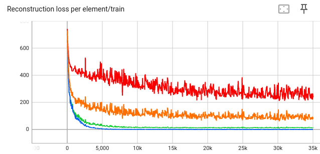
Conversely, a larger \(\lambda\) causes the L2 reconstruction loss to be worse:
How do we choose which of these four models is the right one? Anthropic trained three sparse autoencoders, which each satsified this condition:
For all three SAEs, the average number of features active (i.e. with nonzero activations) on a given token was fewer than 300
So we can plot this value on the training set over time.
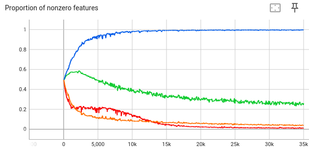
In particular, the values at step 35k are:
- For \( \lambda = 0 \): proportion = 0.9959, so there are 9959 active features
- This isn’t surprising—with no sparsity penalty, the autoencoder can use all the features to minimize reconstruction loss.
- For \( \lambda = 5 \): proportion = 0.2484, so there are 2484 active features
- For \( \lambda = 50 \): proportion = 0.03829, so there are ~383 active features
- For \( \lambda = 500 \): proportion = 0.01068, so there are ~107 active features
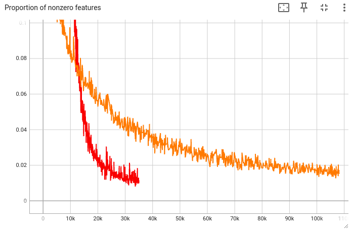
If we zoom in, we see that the proportion is still decreasing:
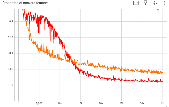
As a rough guide, I want this proportion to be under 300, but not too far—else the L1 penalty might be too strong. So let’s choose \( \lambda = 50 \) and train until step 105k, in the hope that the metric goes under 300.
(I’m choosing the number of steps so that it trains on a few hours on my laptop.)
And that’s what happens: At step 105k, there are roughly 156 active features:
Step 105k is the checkpoint I’ll use for downstream experiments.
Comparing dataset size
At step 105k, the model has seen 2.29e7 tokens. Anthropic purposely left number of tokens off their graph, but in their previous work they trained for 8e9 tokens with much smaller models. (Note that I’m training on consecutive tokens, whereas they sampled and shuffled first.)
Anthropic says
As the compute budget increases, the optimal allocations of FLOPS to training steps and number of features both scale approximately as power laws. In general, the optimal number of features appears to scale somewhat more quickly than the optimal number of training steps
Since in the previous post their largest model had 1.3e5 parameters, while in “Scaling Monosemanticity” their largest model had 3.4e7 parameters, I estimate that the dataset scaled up also by roughly 100x, so I’d guess they trained their largest autoencoder on very roughly 1e12 tokens.