Training an autoencoder
Let’s forget about the sparse part for now. What we want is an autoencoder: a neural network that takes some input and tries to outputs the same thing.
Q: That sounds like it’s trying to do nothing.
A: Yes, but the autoencoder does it in a complicated way. More on this below
What’s the input?
Anthropic trained on the activation after a middle layer of Claude:
we focused on applying SAEs to residual stream activations halfway through the model (i.e. at the “middle layer”).
They have various justifications for this. My intuition is that the middle layer is maybe where the model is thinking the most about concepts, because at the front and back it has to think more about processing input and preparing output, respectively. (See also this paper: “the middle layers [focus] on more abstract patterns”.)
TinyStories-33M has
4 transformer layers. So we
take the activation after the 2nd
layer, while feeding it short stories
from the roneneldan/TinyStories dataset.
This is a vector in \( \mathbb{R}^{768} \),
i.e. a list of activation strengths, one for each of 768 neurons.
What’s the autoencoder?
If the autoencoder did nothing, that would be
def autoencoder(llm_activations):
    return llm_activations
It’s a little more complicated than that:
def autoencoder(llm_activations):
    features = relu(encoder_linear(llm_activations))
    return decoder_linear(features)
In this function:
- ReLU maps negative elements to 0
encoder_linearis an affine transformation \( x \mapsto Ax+b \), where \(A\) is the weight matrix and \(b\) is the bias vectordecoder_linearis another affine transformation (with different weight \(C\) and bias \(d\))
Q: Why does this have the fancy name autoencoder? It’s just a standard MLP.
A: Because there are some more constraints:
encoder_linearis \( \mathbb{R}^{768} \to \mathbb{R}^F \), where F is the hidden dimension (F for number of Features) of the autoencoder. That is,encoder_lineartakes a vector with 768 elements, and spits out a vector with F elementsdecoder_linearis \( \mathbb{R}^{F} \to \mathbb{R}^{768} \). So the net effect is thatautoencoderreturns a vector with the same dimension as the input vector
We’d like activations and autoencoder(activations) to be as close together
as possible (“auto” means “self”, not “car”).
This won’t happen by default, since encoder_linear and decoder_linear
are random transformations.
But we can quantify how far apart they are using an L2 norm:
reconstruction_loss = ((activations - autoencoder(activations)) ** 2).sum()
And then we can use gradient descent to adjust the weights and biases of the autoencoder to minimize the reconstruction loss.
Training
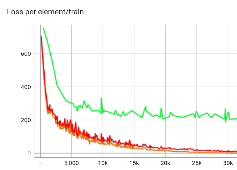
Let’s train autoencoders with different numbers of features:
- \(F=100\) (green)
- \(F=767\) (blue)
- \(F=768\) (red)
- \(F=1000\) (orange)
We’ll save checkpoints every 5000 steps because we’ll do some inference later.
Pytorch makes it easy to save models
using torch.save(model, path).
This is a bad idea.
If you later move the import class to a different file, you may not be able to load old checkpoints. Did I know this anyway but still walk into this footgun? Yes.
The safe
but clunkier way is
torch.save(model.state_dict(), path).
Graph of the reconstruction loss over time:

The blue curve is difficult to see because it’s almost perfectly covered by red.
All the curves converge to 0 loss, except for \(F=100\).
This makes sense: If you have to compress a vector in \( \mathbb{R}^{768} \) to a vector in \( \mathbb{R}^{100} \), you’re going to lose a lot of information that you can’t recover when decompressing.
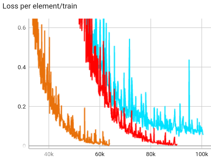
Let’s zoom in on the x-axis:

Here we see that
\(F=767\)
isn’t actually converging to 0;
it gets stuck around loss = 0.1.
We can also explain this: projecting from \( \mathbb{R}^{768} \) to \( \mathbb{R}^{767} \) (and back) loses just a little information.